Path Finder using a Recursive Process – Example 8.5

February 17, 2015

A not uncommon task for Landscape designers is to draw paths through the landscape. If you are working on a “flat site” (something which doesn’t exist) or if you are just deciding to ignore topography completely, you can just draw the paths anywhere in any configuration you want. This will lead to problems.

Anyone who has a basic training in site design will know that a path cannot legally exceed a slope of 1:12 for general accessibility (and then only with occasional, unsightly flat spots). A better rule of thumb is to have no path exceed 1:20 as this is a maximum slope that is generally comfortable for the largest range of the population. An unpaved trail can have a slope up to 1:10 to allow use by an off-road wheelchair, and in special cases, trails which are not accessible may exceed this gradient, but ideally not for prolonged distances as prolonged walking becomes difficult.

I had tried out several variations of a script that could generate a range of paths that meet these certain requirements, and one of the better solutions I’ve come up with so far uses a recursive process to figure out an acceptable path. I was inspired by a story I heard about ancient road builders who would determine where to put a path or road by setting an animal loose (a goat maybe) and letting it find the ideal gradient across a pass, etc. So this script makes the process a bit more efficient and a bit less romantic, but uses a similar logic to create a possible path in incremental steps.

Step One – Initial Setup

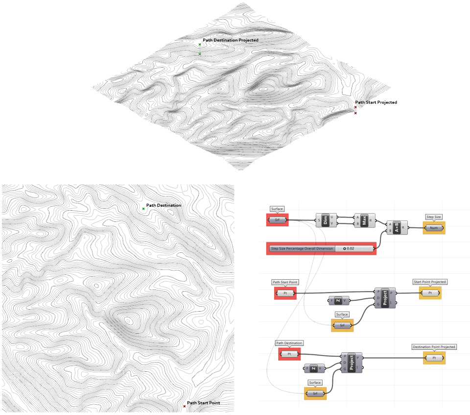
Before starting the script, you will need a topographic surface. This could be a small site, or a large scale landscape. We will allow the script to scale itself to the landscape in question. In this particular case, I generated a 5km x 5km terrain using the process described in Example 20.2 of an area around Grünenplan, Niedersachsen in Germany, although this isn’t important… any area will do. I then draw two points in 2D Space in Rhino, one for the Start of the path and one for the end.

The initial grasshopper steps are also straightforward. First I am measuring the dimensions of my surface and multiplying this by a factor to determine my growth interval. The resulting number “Step Size” is put into its own container that I can copy to future steps. Having a step sized as a proportion of the overall surface size will allow the script to better adapt to different sizes of terrain. The other thing I need to do in Grasshopper is to use “Project Point” to project my Geometry, the Start and Destination points, to the surface.

Step Two – Starting the Loop and Finding a Range of Possible Path Directions

Whenever you set up a loop, several questions need to be answered. What do I want to achieve, and how do I structure my data to achieve this? There are always multiple possibilities, and with experience you will tend to favor certain ways over others. In this particular case, I will use the D0 data stream for the “active” or leading point in my growing path, do some operations to determine the next point in my path, and will then “archive” previous points in the path in a growing list of points kept in the D1 data stream. From the beginning, however, I will insert my starting point into both the D0 and D1 streams since I want to use this point as both my active point, as well as archive it. This should make sense later.

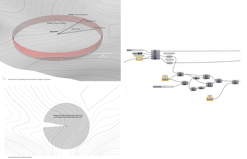
Once I have my data streams setup, there are two basic steps the loop will execute. In this first step, the script will find a range of possible path directions based on an allowable path rise/fall that is adjustable. This is achieved by dividing the variable “Step Size” by a factor. So for a 1:12 slope (8.3%) if the path is traveling 20m in the horizontal direction, it can travel only 1.67m either up or down and to stay within the acceptable range. We are going to solve this geometrically. First we create a circle circle with its center point at our current path endpoint (the position of our wandering goat), and with a radius equal to our “Step Size”. We then copy this circle both up and down with a distance equal to our allowable rise/fall. We then create a “Loft” between the upper and lower circles. Finally, we use the Brep to Brep Intersect component  (BBX) to find where the Terrain Surface and the Surface between the circles intersects. This generates one or more curves which represent acceptable locations for the next point on our path. In the particular example above, this curve is represented with a white dashed line, and nearly every point on the circle, except for a small pie slice, could produce a path with an acceptable slope.

Step Three – Deciding on the “Best” possible Next Point for the Path

If the Curve output from the “BREP to BREP Intersect” component represents the range of possible or allowable next steps in the path, we need a criteria to decide which of these possible points we actually want to use. In this case, since we have a destination we are trying to get to, we will assume that the point closest to this ultimate destination is the “best”. To get this point, the script uses two closest point components. The first of these, “Curve Closest Point” finds the point on each of the curves output from “BBX”. If there is only one curve, as in the image from Step two, only one point would be output from the component and we could move on. For this reason, I’ve advanced the loop a few steps to show an instance where BBX outputs two distinct curves. (more than 2 curves are also possible) Again, the grey pie slices represent allowable path directions, the range in which the path would not rise or fall too much. When the two curves associated with these grey slides are tested with “Crv CP”, two points are produced.

We now need one more component, “Closest Point” to decide which of these two components if indeed the closest to the final destination point. In this case, the point indicated in green, to the left, happens to be the closest point, as opposed to the red point on the right. This is a propitious moment, as the path will now go around the central mountain in a clockwise direction, as opposed to the other possibility of a counterclockwise heading.

Step Four – Finishing the Loop

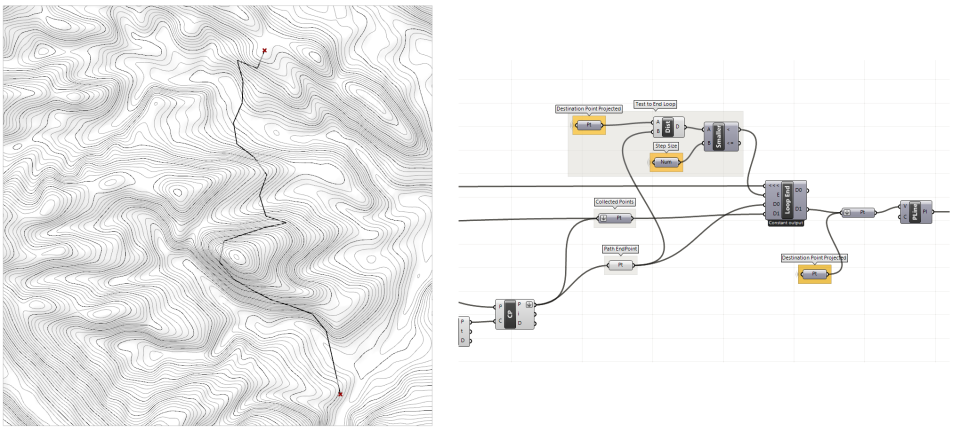
The next point for our path is now determined, labeled “Path End Point” and I will add this point both to the end of my growing list of collected points kept in the D1 data stream, and will also input it into the D0 stream to replace the initial point placed in D0 at the start. D0 will therefore always only have one point in it, while the list length of D1 will be equal to the number of steps the loop runs to get from the start to the destination. I don’t know yet how many steps this will be, but once I get there, I want my loop to stop otherwise the list will keep senselessly growing. That is why I have an escape test, which tests the distance between the “Path End Point” and the “Destination Point Projected.” If this distance is less than our overall “Step Size”, we have arrived, or rather our goat has arrived, and everyone can celebrate. A “True” value is returned from the Boolean test and the loop ends.

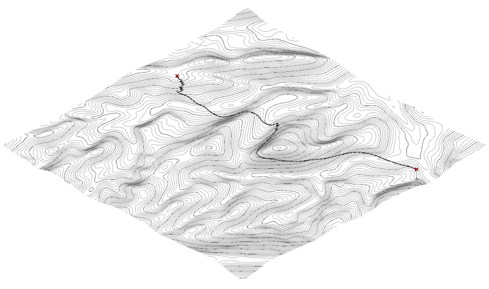
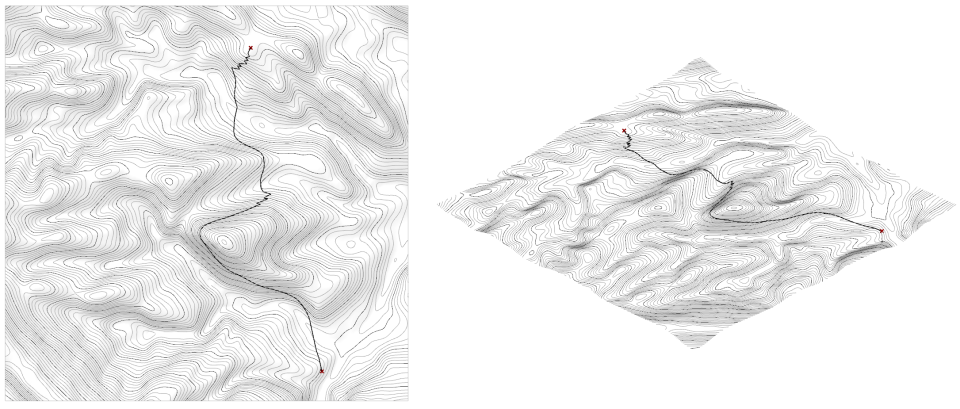
After the loop, the list of points generated in D1, the overall journey of our goat, is stitched together with a polyline to create the path. The image above represents this completed path.

In the test phase, I was using a rather large step size (.05), or 5% of the overall dimension of the study area to draw my path. For a smoother path, I might want to use a smaller step size. The second image above represents a path drawn between the two points with a 1% step size. While the overall vector remains similar, you’ll notice the smaller step size also creates smaller switchbacks.

Variations and Other Possibilities

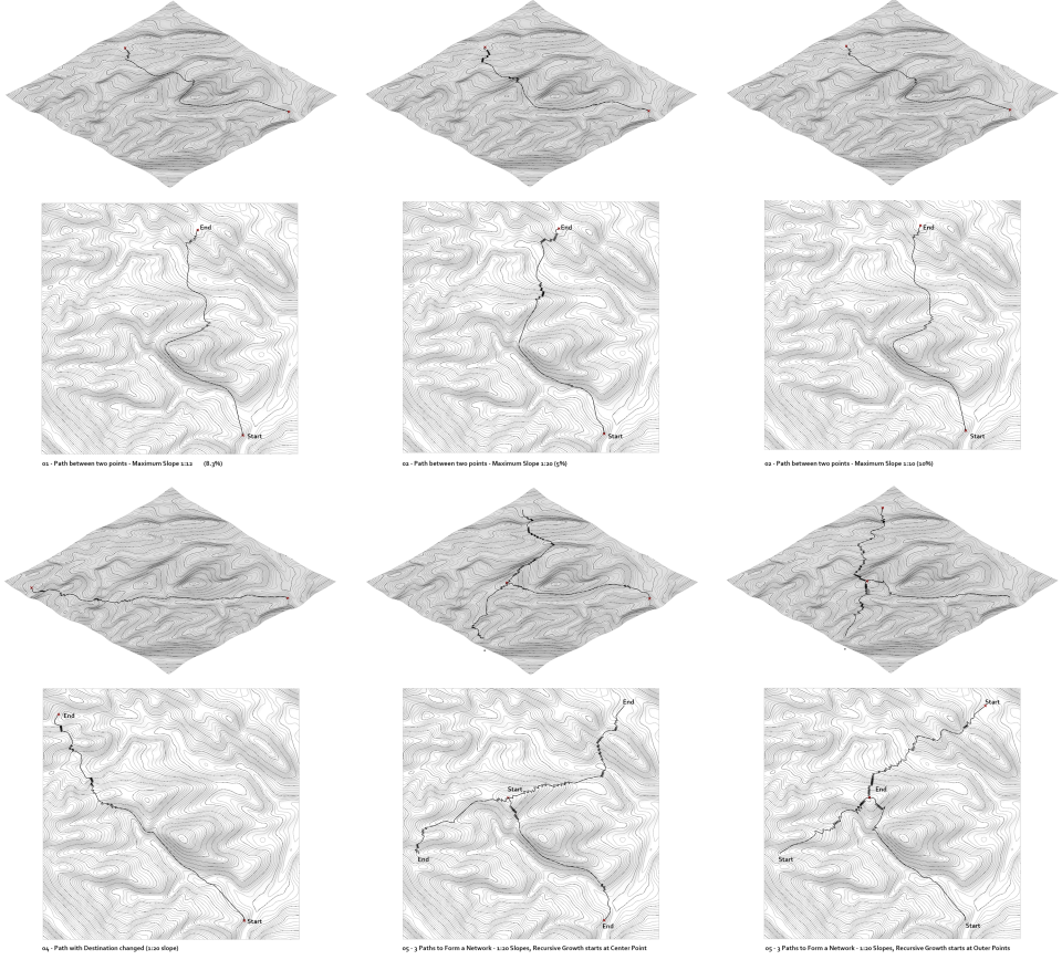
The image above represents a few things you can now try out with the script. The first thing is to change the path’s allowable slope. The top three images represent 3 maximum slope possibilities.

The second thing to do is simply change the start and destination points. The pathfinder in each case tries to find an acceptable course. You can link several of these studies together to start to create a path network.

One last thing to note, determining where the path “Starts” vs. “Ends” will have an effect on the path’s final form. In image 5 above, all the paths start at a summit and work their way to a series of outer points. In Image 6, the paths start at the outer points, and work their way to the summit. You’ll notice in the top right path, when it starts at the summit, the pathfinder uses the natural ridge to work its way down and towards its destination. When the pathfinder is reversed, the opportunity to use this natural ridge is lost since the pathfinder was a bit short sighted, and now has no other choice but to approach the summit through a grueling set of switchbacks up the North Face.

Post navigation

← Example 11.4 – Simple Agent to Agent Interaction

Købmagergade, Copenhagen – Karres en Brands – Case Study 3 →