Fractal Trees – Basic L-System- Example 9.4

October 7, 2014

Another very useful application for fractal processes is to create 3D vegetation for your models. There are several very good commercial products which use algorithms to create plants, which combine mathematical understanding with botanical knowledge to make tree and plant generators. Two popular products that I have a little experience with are Xfrog and Laubwerk, both initially developed by German programmers. While the goal of this post is not to get you to recreate their software, understanding some of the basic principles can help you use either one more intelligently (if you want or need high quality plants for renderings), but can also serve as an inspiration for potential design applications which go beyond rendering and representation. Also, creating your own simple tree generator, combined with a smart use of a random seeds can allow you to make basic ‘stick’ models of plants that don’t look repetitive and which can give an impression of vegetation quality and massing without being too photo-realistic.

A core family of algorithms in these plant generators are ‘L-systems’, or Lindenmayer systems. You can read about these to get a general sense of the mathematical theory but I find the best way to start to understand them is to do a few yourself. A useful plugin for Grasshopper that works with L-systems is one called Rabbit by Morphocode, but I will show you 4 simple L-systems that can be easily developed without Rabbit using only Grasshopper and Anemone, and from there maybe you can experiment with your own. Another useful source for starting to develop your own L-systems is the book “The Algorithmic Beauty of Plants” which you can download for free via PDF, a product of the research Institute Algorithmic Botany at the University of Calgary. Some of my examples are explained in this book in more detail.

Like the fractal systems we looked at previously, L systems have a set of production rules, which are repeated through a few recursions or generations. Each generation starts drawing a structure at a starting point, and draws lines at defined angles and lengths. Each subsequent generation draws a similar structure at new starting points that were defined in the previous generation.

Probably the simplest L-system is One where you take a point, and draw two lines, one at a positive vector angle, and one negative (the angle is a variable). The length of the line is proportionally reduced in each generation.

Basic ‘L’-System Production rules and results after two and three generations.

With these production rules, after each generation the number of Lines doubles. By varying the angle of branching and the proportion of reduction for each generation, though, the formal expression of the production rules can be quite different. I coded these production rules in an Anemone loop in Grasshopper, and after a fixed number of generations (much more than 7 or 8 generations will be overkill!) it draws pipes along each line with the radius of the Pipe based on the overall length of the line. Script image to follow a bit later…

The above image shows how one of these systems can radically change with various angles ranging between 15° and 90°. As you can see, the angles much above maybe 30° don’t look like real plants but between 15° and 30° they can look surprisingly life-like, especially considering the sheer simplicity of the system.

The script should be easy to develop if you have been following along with the previous exercises and if you’re a somewhat capable user of Grasshopper. The ‘L’ system is developed in the blue part of the script.

Various plants have self-similar, repeating logics that define their structure. If you have studied plant botany and tree identification, you will know some species have branches that alternate, some where two branches always come from the same spot, etc. Understanding potential structures can allow you to modify the system.

Three potential variations on the basic ‘L’ system

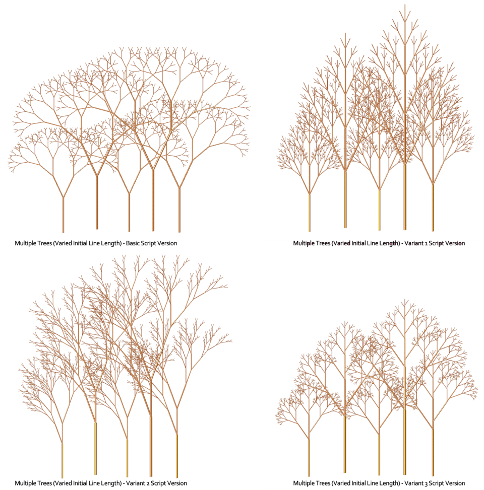
In the image above, I show three variants to my initial script. In the first, Instead of drawing two lines to loop, I draw three, one going straight. The other two variations have slightly more complex branching structures, but should be easy to code if you understand the system.

Variation can be created by varying the initial line length.

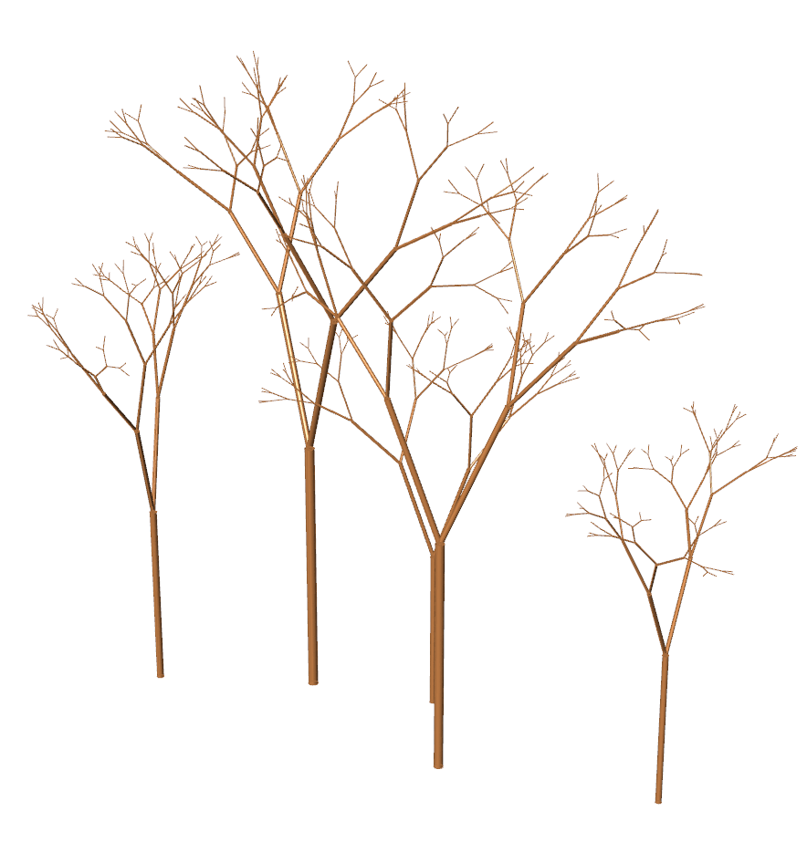
Trees in nature also follow basic rules, with variation in growth created by factors such as soil composition, sunlight, adjacencies, and genetic chance. Once you develop a basic process, you can find ways to introduce variation into the system. Here it is done very simply, just by varying the length of the initial line. You’ll notice the overall structure of each tree is exactly the same though…only the scale is different. More complex variation can be introduced with things like random number generators. In a future example, I will show the creation of a 3D tree using a random number generator that gives a possible range of branching angles, plus a system for rotating the branches in the 3rd dimension. The results of my initial test are shown in the image below, but you’ll have to wait for the explanation…or try and figure it out yourself! 🙂 The only hint I will give you is you have to really pay attention to your data structures!

Basic ‘L’ system with branches rotated in the 3rd dimension, and with angles allowed within a defined range of random numbers.

Post navigation

← Adding Detail to a Region – Forests – Example 20.6

Vector Field Tools in Grasshopper – Basic + and – Point Charges – Example 7.1 →